How to Build a Custom Embedded Stereo System for Depth Perception
There are various 3D sensor options for developing depth perception systems including, stereo vision with cameras, lidar, and time-of-flight sensors. Each option has its strengths and weaknesses. A stereo system is typically low cost, rugged enough for outdoor use, and can provide a high-resolution color point cloud.
There are various off-the-shelf stereo systems available on the market today. Depending on factors such as accuracy, baseline, field-of-view, and resolution, there are times when system engineers need to build a custom system to address specific application requirements.
In this article, we first describe the main parts of a stereo vision system then provide instructions on making your own custom stereo camera using off-the-shelf hardware components and open-source software. As this setup is focused on being embedded, it will compute a depth map of any scene in real-time, without the need of a host computer. In a separate article, we discuss how to build a custom stereo system to use with a host computer when space is less of a constraint.
Another application that can greatly benefit from such an onboard processing system is object detection. With advances in deep learning, it has become relatively easy to add object detection to applications, but the need of dedicated GPU resources makes it prohibitive for many users. In this article, we also discuss how to add deep learning to your stereo vision application without the need of an expensive host GPU. We have divided the sample code and sections of this article into stereo vision and deep learning, so if your application does not require deep learning, feel free to skip the deep learning sections.
Stereo Vision Overview
Stereo vision is the extraction of 3D information from digital images by comparing the information in a scene from two viewpoints. Relative positions of an object in two image planes provides information about the depth of the object from the camera.
An overview of a stereo vision system is shown in Figure 1 and consists of the following key steps:
- Calibration: Camera calibration refers to both the intrinsic and extrinsic The intrinsic calibration determines the image center, focal length, and distortion parameters, while the extrinsic calibration determines the 3D positions of the cameras. This is a crucial step in many computer vision applications especially when metric information about the scene, such as depth, is required. We will discuss the calibration step in detail in Section 5 below.
- Rectification: Stereo rectification refers to the process of reprojecting image planes onto a common plane parallel to the line between camera centers. After rectification, corresponding points lie on the same row, which greatly reduces cost and ambiguity of matching. This step is done in the code provided to build your own system.
- Stereo matching: This refers to the process of matching pixels between the left and right images, which generates disparity images. The Semi-Global Matching (SGM) algorithm will be used in the code provided to build your own system.
- Triangulation: Triangulation refers to the process of determining a point in 3D space given its projection onto the two images. The disparity image will be converted to a 3D point cloud.
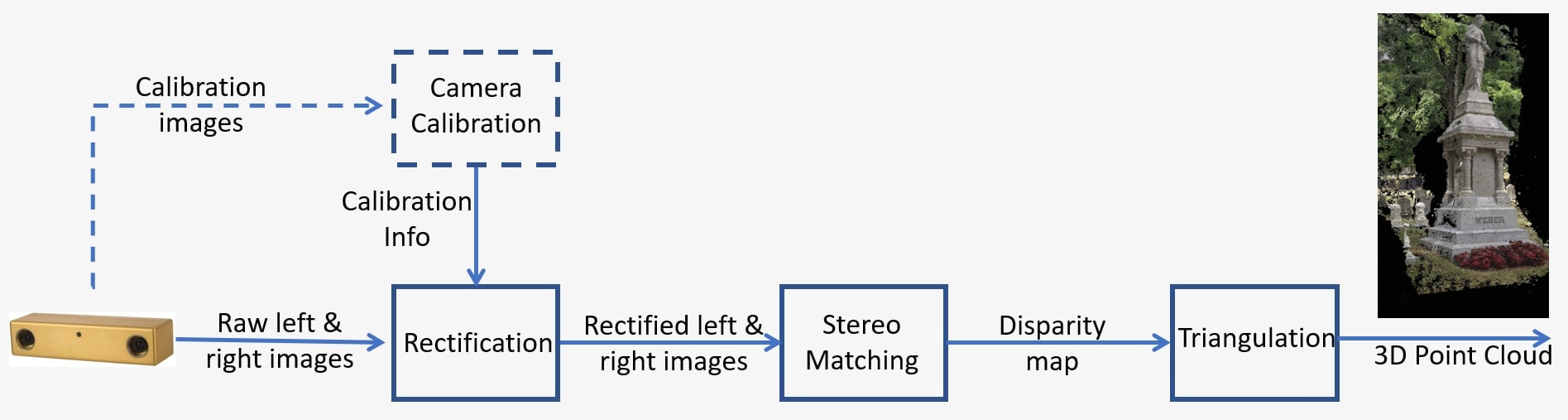
Figure 1: Overview of a stereo vision system
Deep Learning Overview
Deep learning is a subfield of machine learning that deals with algorithms inspired by the structure and function of the brain. It tries to mimic the learning capability of the human brain. Deep learning algorithms can perform complex operations such as object recognition, classification, segmentation, etc efficiently. Amongst other things, deep learning enables the machines to recognize people and objects in the images fed to it. The particular application we are interested in is people detection. Training your own deep learning algorithms require a large amount of labelled training data but open-source pre-trained models makes it easier for anyone to develop these applications.
Deep learning also requires high performance GPUs but the Quartet solution for TX2 comes with all the capabilities of a larger GPU at a fraction of the form factor and power consumption. Having the deep learning models running on the TX2 also has the added benefit of mobility and is a perfect candidate for mobile robots that need to detect people to steer clear of them.
Design Example
Let’s go through a stereo system design example. Here are the requirements for a mobile robot application in a dynamic environment with fast moving objects. The scene of interest is 2 m in size, the distance from the cameras to the scene is 3 m and the desired accuracy is 1 cm at 3 m.
You can refer to this article for more details on stereo accuracy. The depth error is given by: ΔZ=Z²/Bf * Δd which depends on the following factors:
- Z is the range
- B is the baseline
- f is the focal length in pixels, which is related to the camera field-of-view and image resolution
There are various design options that can fulfill these requirements. Based on the scene size and distance requirements above, we can determine the focal length of the lens for a specific sensor. Together with the baseline, we can use the formula above to calculate the expected depth error at 3 m, to verify that it meets the accuracy requirement.
Two options are shown in Figure 2, using lower resolution cameras with a longer baseline or higher resolution cameras with a shorter . The first option is a larger camera but has lower computational need, while the second option is a more compact camera but has a higher computational need. For this application, we chose the second option as a compact size is more desirable for the mobile robot and we can use the Quartet Embedded Solution for TX2 which has a powerful GPU onboard to handle the processing needs.
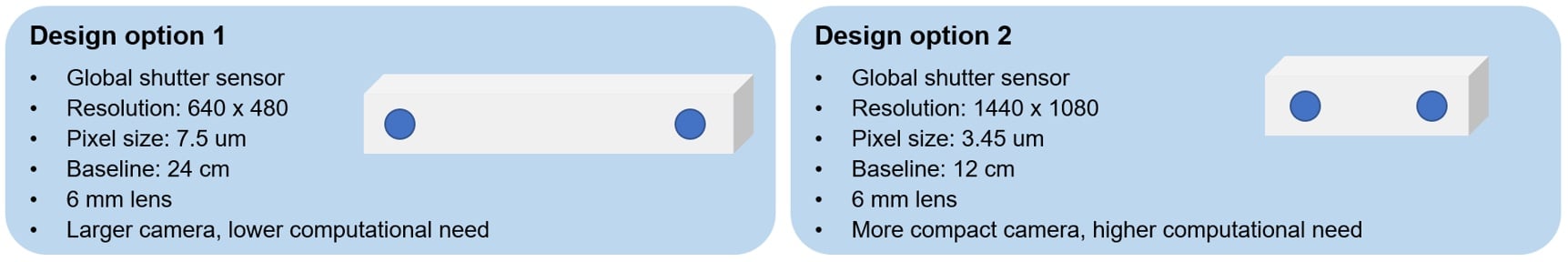
Figure 2: Stereo system design options for an example application
Hardware Requirements
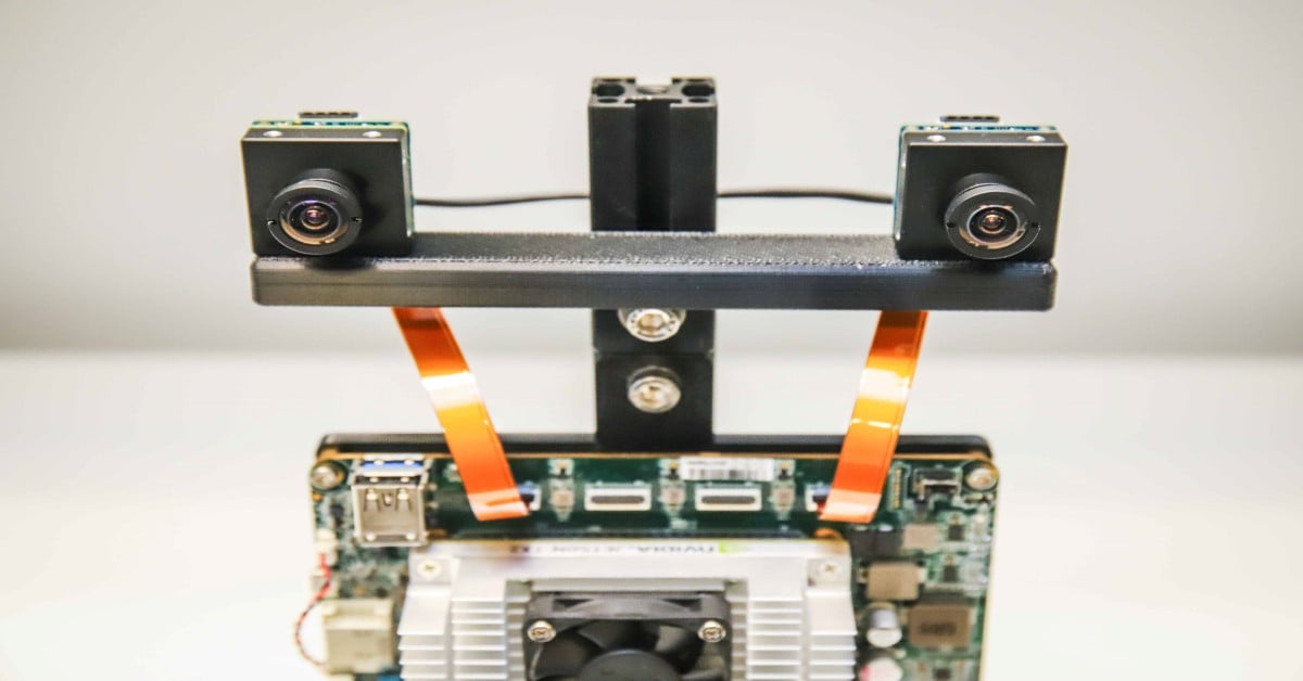
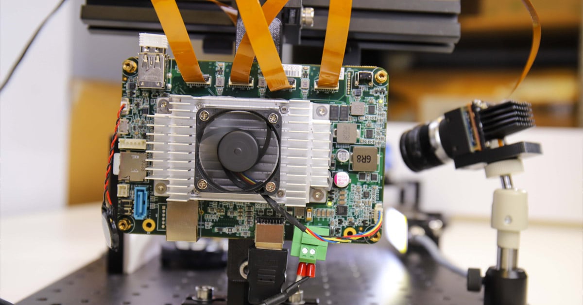
For this example, we mount two Blackfly S board level 1.6 MP cameras using the IMX273 Sony Pregius global shutter sensor on a 3D printed bar at 12 cm baseline. Both cameras have similar 6 mm S-mount lenses. The cameras connect to the Quartet Embedded Solution for TX2 customized carrier board using two FPC cables. To synchronize the left and right camera to capture images at the same time, a sync cable is made that connects the two cameras. Figure 3 shows the front and back views of our custom embedded stereo system.
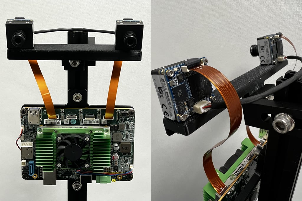
Figure 3: Front and back views of our custom embedded stereo system
The following table lists all the hardware components:
|
Part |
Description |
Quantity |
Link |
|
ACC-01-6005 |
Quartet Carrier with TX2 Module 8GB |
1 |
https://www.flir.com/products/quartet-embedded-solution-for-tx2/ |
|
BFS-U3-16S2C-BD2 |
1.6 MP, 226 FPS, Sony IMX273, Color |
2 |
|
|
ACC-01-5009 |
S-Mount & IR filter for BFS color board level cameras |
2 |
|
|
BW3M60B-1000 |
6 mm S-Mount Lens |
|
http://www.boowon.co.kr/site/ |
|
ACC-01-2401 |
15 cm FPC cable for board level Blackfly S |
2 |
https://www.flir.com/products/15-cm-fpc-cable-for-board-level-blackfly-s/ |
|
XHG302 |
NVIDIA® Jetson™ TX2/TX2 4GB/TX2i Active Heat Sink |
1 |
https://connecttech.com/product/nvidia-jetson-tx2-tx1-active-heat-sink/ |
|
Synchronization cable (make your own) |
1 |
||
|
Mounting bar (make your own) |
1 |
Both lenses should be adjusted to focus the cameras on the range of distances your application requires. Tighten the screw (circled in red in Figure 4) on each lens to keep the focus.
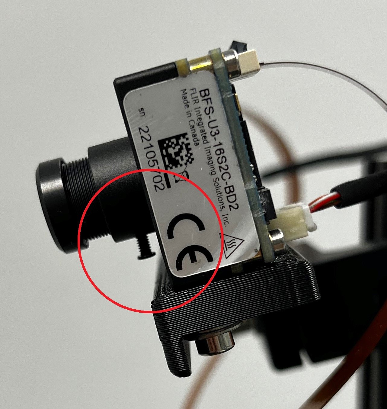
Figure 4: Side view of our stereo system showing the lens screw
Software Requirements
a. Spinnaker
Teledyne FLIR Spinnaker SDK comes pre-installed on your Quartet Embedded Solutions for TX2. Spinnaker is required to communicate with the cameras.
b. OpenCV 4.5.2 with CUDA support
OpenCV version 4.5.1 or newer is required for SGM, the stereo matching algorithm we are using. Download the zip file containing the code for this article and unzip it to StereoDepth folder. The script to install OpenCV is OpenCVInstaller.sh. Type the following commands in a terminal:
- cd ~/StereoDepth
- chmod +x OpenCVInstaller.sh
- ./OpenCVInstaller.sh
The installer will ask you to input your admin password. The installer will start installing OpenCV 4.5.2. It may take a couple of hours to download and build OpenCV.
c. Jetson-inference (if deep learning is needed)
Jetson-inference is an open-source library from NVIDIA that can be used for GPU-accelerated deep learning on Jetson devices, like the TX2. The library makes use of the TensorRT SDK which facilitates high performance inference on NVIDIA GPUs. Jetson-inference provides the user an array of pre-trained and ready to use deep learning models and the code to deploy these models using TensorRT. To install jetson-inference, type the following commands in a terminal:
- cd ~/StereoDepth
- chmod +x InferenceInstaller.sh
- ./InferenceInstaller.sh
Calibration
The code to grab stereo images and calibrate them can be found in the “Calibration” folder. Use the SpinView GUI to identify the serial numbers for the left and right cameras. For our settings, the right camera is the master and left camera is the slave. Copy the master and slave camera serial numbers to file grabStereoImages.cpp lines 60 and 61. Build the executable using the following commands in a terminal:
- cd ~/StereoDepth/Calibration
- mkdir build
- mkdir -p images/{left, right}
- cd build
- cmake ..
- make
Print out the checkerboard pattern from this link and attach it to a flat surface to use as the calibration target. For best results while calibrating, in SpinView set Exposure Auto to Off and adjust the exposure so the checkerboard pattern is clear and the white squares are not over exposed, as shown in Figure 5. After the calibration images are collected, gain and exposure can be set to auto in SpinView.
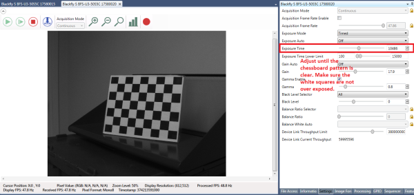
Figure 5: SpinView GUI settings
To start collecting the images, type
- ./grabStereoImages
The code should start collecting images at about 1 frame/second. Left images are stored in images/left folder and right images are stored in images/right folder. Move the target around so that it appears in every corner of the image. You may rotate the target, take images from close by and from further away. By default, the program captures 100 image pairs, but can be changed with a command line argument:
- ./grabStereoImages 20
This will collect only 20 pairs of images. Please note this will overwrite any images previously written in the folders. Some sample calibration images are shown in Figure 6.
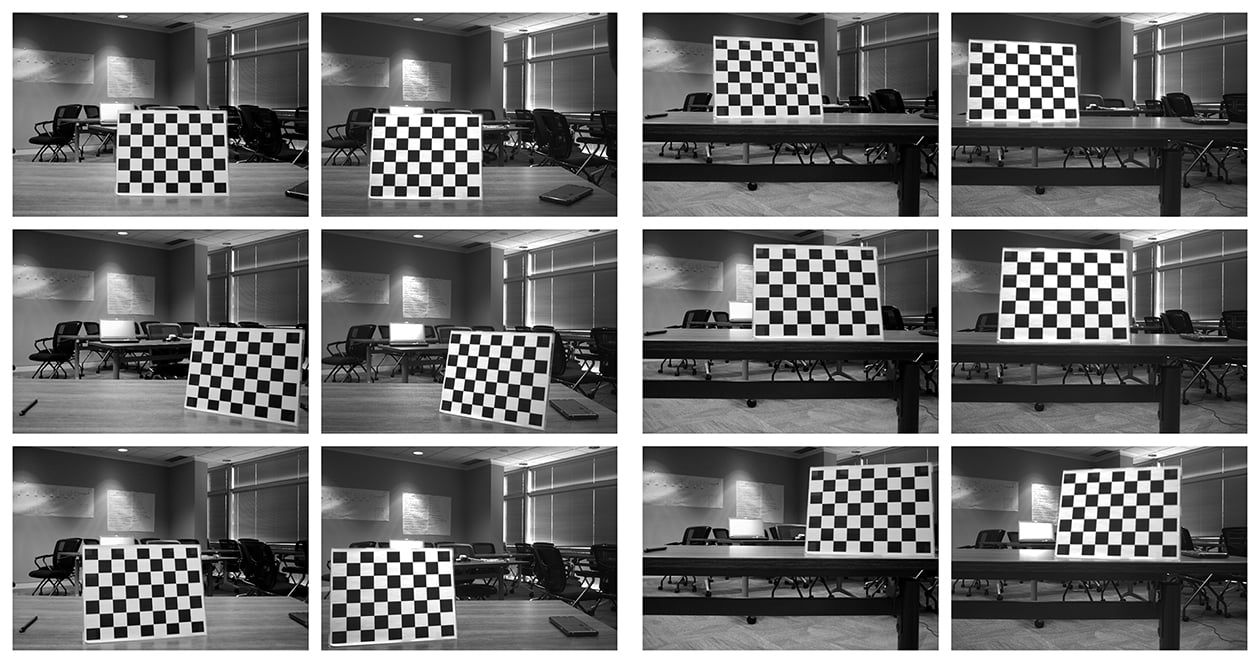
Figure 6: Sample calibration images
After collecting the images, run the calibration Python code by typing:
- cd ~/StereoDepth/Calibration
- python cameraCalibration.py
This will generate 2 files called “intrinsics.yml” and “extrinsics.yml” which contain the intrinsic and extrinsic parameters of the stereo system. The code assumes 30mm checkerboard square size by default but can be edited if needed. At the end of the calibration, it will display the RMS error which indicates how well the calibration is. Typical RMS error for good calibration should be below 0.5 pixel.
Real-time Depth Map
The code to calculate disparity in real-time is in the “Depth” folder. Copy the serial numbers of cameras to file live_disparity.cpp lines 230 and 231. Build the executable using the following commands in a terminal:
- cd ~/StereoDepth/Depth
- mkdir build
- cd build
- cmake ..
- make
Copy the “intrinsics.yml” and the “extrinsics.yml” files obtained in the calibration step to this folder. To run the real-time depth map demo, type
- ./live_disparity
It would display the left camera image (raw unrectified image) and the depth map (our final output). Some example outputs are shown in Figure 7. The distance from the camera is color-coded according to the legend on the right of the depth map. The black region in the depth map means no disparity data was found in that region. Thanks to the NVIDIA Jetson TX2 GPU, it can run up to 5 frames/second at a resolution of 1440 × 1080 and up to 13 frames/second at a resolution of 720 × 540.
To see the depth at a particular point, click on that point in the depth map and the depth will be displayed, as shown in the last example in Figure 7.
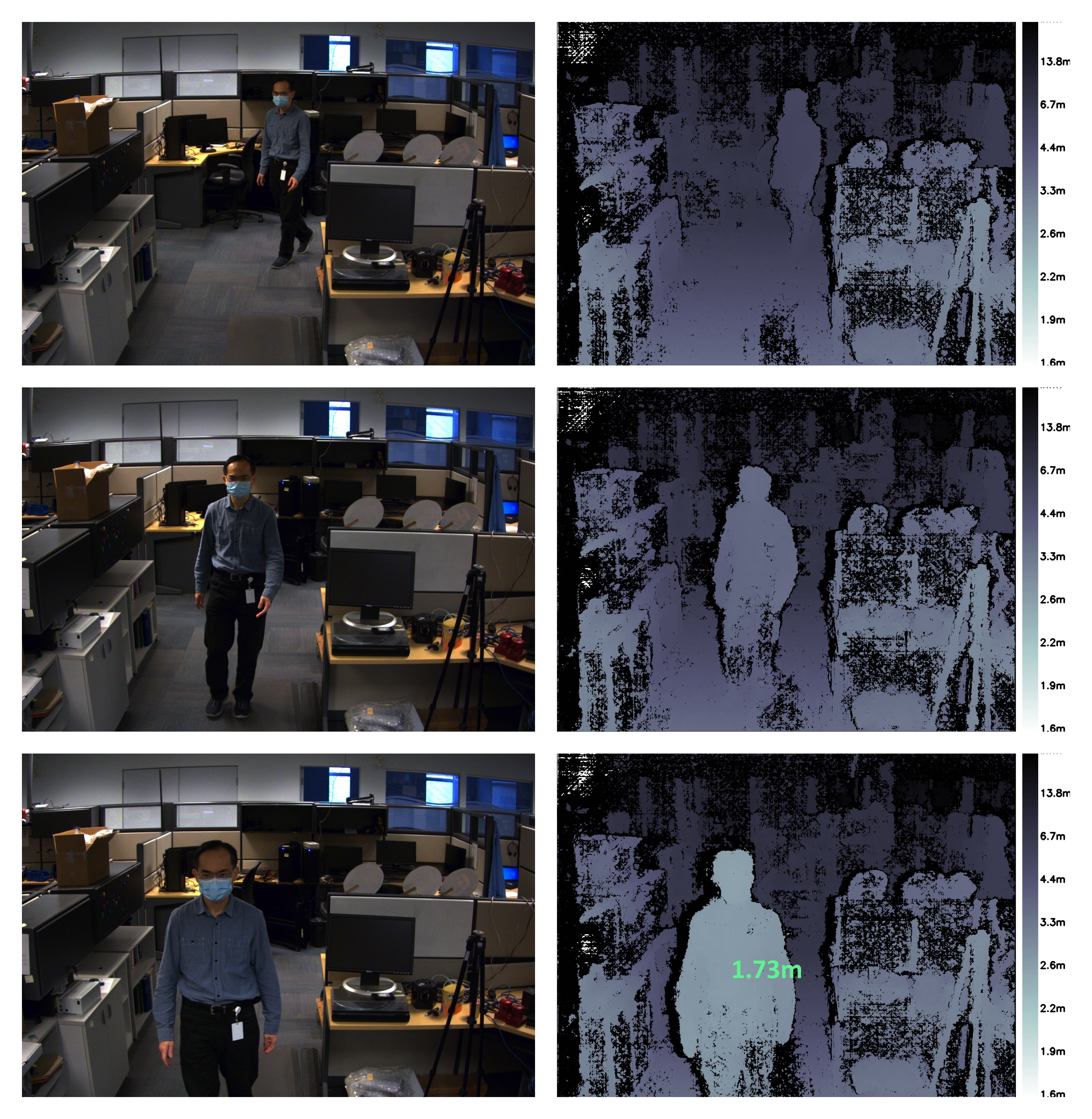
Figure 7: Sample left camera images and corresponding depth map. The bottom depth map also shows the depth at a particular point.
Person detection
We use DetectNet provided by Jetson-inference to detect humans in an image frame. DetectNet comes with options to select the deep learning model architecture for object detection. We use the Single Shot Detection (SSD) architecture with a MobileNetV2 backbone to optimize for both speed and accuracy. When running the demo for the first time, TensorRT creates a serialized engine to further optimize for inference speed, which can take a few minutes to complete. This engine is automatically saved in files for further runs. The architecture used is quite efficient and one can expect ~50 fps for running the detection module. The code for person detection capability along with stereo depth in real-time is in the “DepthAndDetection” folder. Copy the serial numbers of cameras to file live_disparity.cpp lines 271 and 272. Build the executable using the following commands in a terminal:
- cd ~/StereoDepth/DepthAndDetection
- mkdir build
- cd build
- cmake ..
- make
Copy the “intrinsics.yml” and the “extrinsics.yml” files obtained in the calibration step to this folder. To run the real-time depth map demo, type
- ./live_disparity
Two windows showing the left rectified color images and the depth map will be displayed. The depth map is color-coded for better visualization of the depth map. Both windows have bounding boxes surrounding the people in the frame and show the average distance to the person from the camera. With both stereo processing and deep learning inference, the demo runs at around ~4 fps at a resolution of 1440 × 1080 and up to 11.5 fps for a resolution of 720 × 540.

Figure 8: Sample left camera images and corresponding depth map. All the images show the person detected in the images and the distance of the person from the camera
The people detection algorithm is capable to detecting multiple people even in challenging conditions like occlusion. The code calculates the distances to all the people detected in the image, as shown below.

Figure 9: Left image and the depth map shows multiple people being detected in the image, and their corresponding distance from the camera.
Summary
Using stereo vision to develop a depth perception has the advantages of working well outdoors, the ability to provide a high-resolution depth map, and very accessible with low-cost off-the-shelf components. Depending on the requirements, there are a number of off-the-shelf stereo systems on the market. Should it be necessary for you to develop a custom embedded stereo system, it is a relatively straightforward task with the instructions provided here.
Related Articles
-
Embedded Vision
How to Build a Custom Embedded Stereo System for Depth Perception
Learn more -
 Embedded Vision
Streaming 4x Cameras with Small Carrier Board: Fast Prototype
Read the Story -
 Embedded Vision
Guide for Integrating Board Level Cameras
Read the Story