Overview of the Ladybug Image Stitching Process
Overview
The following diagram provides a high-level overview of the steps required to produce a panoramic image from Ladybug raw image output. The table below briefly explains the steps. The sections that follow explain the Color Processing and Stitching steps in more detail. The final section explains stitching errors and how to work with them.

Figure 1: Ladybug Panoramic Imaging Process
Imaging Step |
Description |
|
Image Capture |
Separate images are captured synchronously from each of the camera’s six sensors and undergo processing, including analog-to-digital conversion to raw (Bayer-tiled) format. |
|
JPEG Compression |
JPEG compression is optional. The purpose of this option is to allow for images to be transferred to the PC at a faster frame rate. If compression is disabled, the camera transmits uncompressed images. If compression is enabled, each image is converted into JPEG compressed format before transmission. Images are transmitted to the PC via the interface cable. |
|
Decompression |
Images are decoded back into raw image format for further processing. |
|
Color Processing |
The raw Bayer-tiled images are interpolated to create a full array of RGB images. Following color processing, images are loaded onto the graphics card of the PC for rectification, blending and stitching. |
|
Rectification |
Rectification corrects the barrel distortion caused by the Ladybuglenses. |
|
Projection |
Image textures are mapped to a single 2- or 3-dimensional coordinate system, depending on the projection that is specified. |
|
Blending |
Pixel values in each image that overlap with the fields of adjacent images are adjusted to minimize the effect of pronounced borders. The result is a single, stitched image. |
Table 1: Ladybug Imaging Process Steps
Color Processing
After raw (Bayer-tiled) images are received from the camera, and decompressed if necessary, they are processed into RGB images using one of the color interpolation methods specified. Most of the color processing algorithms available in the Ladybug API are explained in Different Color Processing Algorithms. An additional algorithm, “down sampling,” scales the textures of each image to half their size in dimension (and quarter-size in data), making it the fastest of all the algorithms. However, due to the nature of scaling down, image resolution is reduced.
Also during color processing, an alpha mask value is assigned to each pixel of each image. This value represents the opaqueness of the pixel and is used in the blending stage. Alpha mask values, in turn, are computed based on the Blending Width value that is specified when the application is first started. This value specifies the pixel width on the border of each image within which blending should take place. Alpha mask values for each image are saved as .pgm files in the \Point Grey Research\PGR Ladybug\bin directory. Adjusting the blending width after an application starts results in the creation of new alpha mask files, which can take some time, depending on the configuration of your PC.
Finally, falloff correction, if specified, is applied to the RGB image to compensate for the vignetting effect of the lenses. Vignetting refers to the boundary area of each image appearing dark relative to the center of the image, creating a shadow effect in the stitched image.
The six RGB-textured images are then transferred to the PC graphics card for stitching.
Stitching
The PC graphics card maps the image textures onto polygon meshes. A polygon mesh is a projection of image textures onto polygons whose geometric vertices are arranged in a 2-dimensional or 3-dimensional coordinate system. If the application specifies a spherical view, the polygons are arranged in 3-dimensional coordinates. If the application specifies a panoramic or dome projection, the polygons are arranged in 2-dimensional coordinates.
The following figures are examples of polygon meshes. The first figure is a 2-dimensional mesh. The second figure is a 3-dimensional mesh (for clarity, only five of the six images are shown).
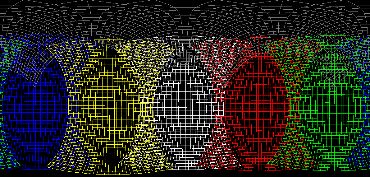
Figure 2: 2-D Polygon Mesh
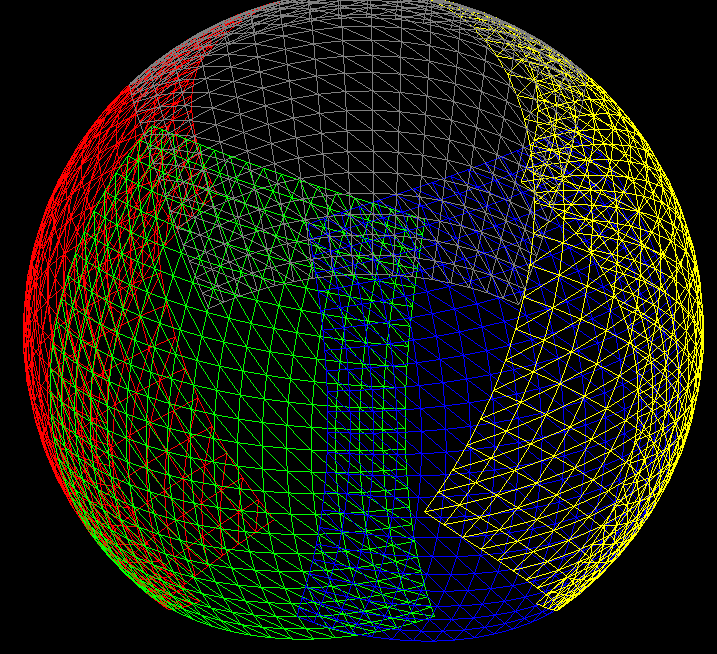
Figure 3: 3-D Polygon Mesh
The coordinates of the polygon meshes are calculated based on calibration data, which specifies how to rectify, rotate and translate images. Because the textures also reflect the alpha values in each pixel, blending from one image to the neighboring image appears smooth. The result is that by transferring image textures to the graphics card, a single, stitched image is produced without consuming any CPU resources.
Dynamic Stitching
Dynamic stitching is a method of adjusting stitching distances along the seam by matching image content. This method may generate better results, but it is very computationally intensive and is not recommended for use during image capture.
Dynamic stitching does not work well if the image has repeating patterns (such as building windows) or a solid color (such as sky).
Users can set the minimum, maximum, and default distance used by dynamic stitching in LadybugCapPro (from the Settings menu, select Options). These settings apply to one-shot and automatic dynamic stitching.
Understanding Stitching Errors
Stitching, Parallax and Calibration Distance
Mapping image textures to polygon meshes means that Ladybug stitching is performed completely based on geometry. As a result, Ladybug stitching is not perfect.
Firstly, the various images that are combined into the panorama are not obtained from exactly the same viewpoint, but from slightly offset viewpoints caused by the physical separation of the individual camera lenses. This effect is known as parallax.
Second, in order to perfectly stitch images together, a range to the physical scene is required. However, since the Ladybug does not do range estimation, we do not have this value. To remove this unknown, we assume all points in the scene are at the same radius from the camera, effectively forcing the real world onto a sphere surrounding the camera.
Current Ladybug cameras are calibrated using a default sphere radius of 20 meters.
|
|
You can change the sphere radius using the sphere size control on the Image Processing toolbar in LadybugCapPro. For details on the options available, see the Ladybug SDK Help or the Technical Reference. |

When the true range is different from the sphere radius, a stitching error results. This error depends upon the separation of the lenses, the sphere radius and the true range. For ranges from 10 meters to infinity, a 20-meter sphere generally results in a parallax error less than 1 pixel in width, and therefore it is a good radius selection for most outdoor scenes.
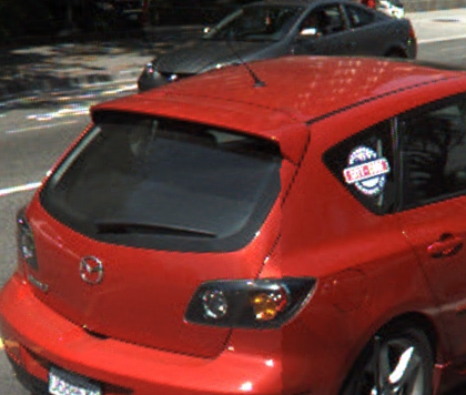
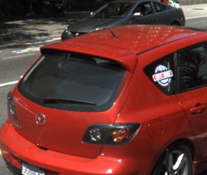
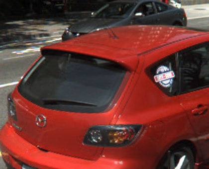
Stitching errors manifest themselves as a ‘double image’ or ’image offset’ effect on the border areas between images. Typically, these errors are most noticeable on objects that are very close to the camera. For example, a ‘double image’ effect can be seen in the following picture:

Figure 4: Image Offset Stitching Error
Slight errors in camera calibration can also contribute to stitching errors.
Some stitching errors can be mitigated by using Dynamic Stitching.
Calculating Stitching Error
You can use the following equation to determine the pixel width within which a stitching error will occur, given the distance between the camera and the subject:
stitching_error (pixels) =![]()
Where:
Z = distance to an object (m)
Zc = calibration distance (m)
K = A constant value determined by the distance between the adjacent camera lenses, focal length and the number of pixels on the sensor.
| Ladybug Camera | Approximate K Value |
| Ladybug6 | 76 for side cameras 104 for the top |
| Ladybug5/Ladybug5+ | 33 for side cameras 54 for the top |
| Ladybug3 | 45 for the side cameras |
| Ladybug2 | 22 for the side cameras |
Note: this is calculated in Ladybug raw pixels so conversion is required if you want to calculate the pixels in the panoramic stitched image.
For example, if the calibration distance is 20 meters, the stitching error that results when an object is an infinite distance from a Ladybug camera is 2.2 pixels.
Stitching and Blending Width
When stitching errors occur, a high blending width value generally results in a more pronounced ‘double image’ effect. A low blending width value, in the presence of stitching errors, generally results in a more pronounced ‘image offset’ effect. When there are no stitching errors—indicating the scene and calibration distance are well-matched—the blending width value has little impact.
In the following series, blending widths of 0, 20, and 100 are applied on images of a nearby subject—approximately three meters from the camera. In the first image, a blending width of 0 renders the border between the stitched images very obvious, which, in turn, makes the offset effect more pronounced. In the second image, a blending width of 20 is specified. This setting still produces an offset error, but it is mitigated somewhat by the blending effect. The third figure specifies a blending width of 100. This setting enhances the offset error, resulting in a ‘double image’ effect.
|
Figure 5: Blending Width=0 |
|
|
Figure 7: Blending Width=100 |
|
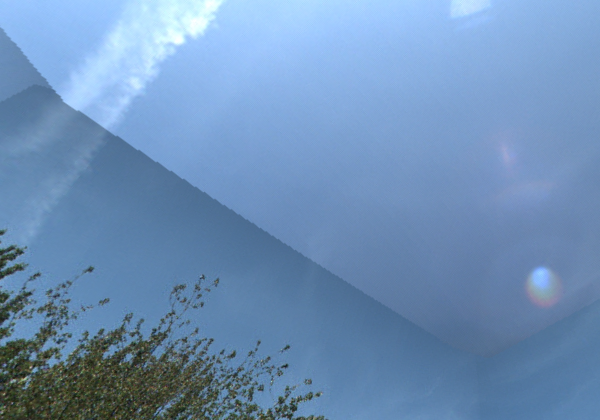
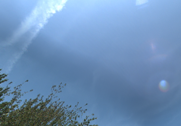
So, when capturing nearby objects, there is a trade-off between blending width and the stitching error effect that you are willing to tolerate in your image. But when capturing distant objects, no parallax-related stitching errors occur, and therefore there is no tradeoff. As seen in the following series of images taken of the sky at blending widths of 0, 20, and 100, the maximum blending width of 100—which is the camera’s default—is clearly the best choice.
|
|
|
|
Figure 10: Blending Width=100 |
|

Stitching and Vignetting
As discussed above, vignetting happens when the boundary area of each image appears dark relative to the center of the image, creating a shadow effect in the stitched image. If you enable falloff correction, the brightness of each image is adjusted so that equally-lit images appear flat in brightness. The side effects of falloff correction are slower processing time due to additional computation, and an amplification of noise in the image.
The following images show the effect of falloff correction. In the first image, falloff correction is disabled; in the second image, falloff correction is enabled.

Figure 11: Falloff Correction Off
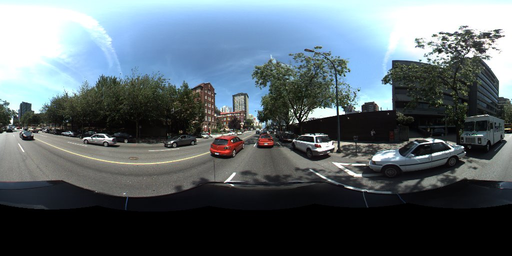
Figure 12: Falloff Correction On